Untitled Document

Introduction to Vortex Lattice Theory

Introducción a la teoría VLM (Vortex Lattice Theory)
Introdução à teoria VLM (Vortex Lattice Theory)

Santiago Pinzón⁴

Recibido: 30/09/2015
Aprobado evaluador interno: 06/11/2015
Aprobado evaluador externo: 27/11/2015

Abstract

Panel methods have been widely used in industry and are well established since the 1970s for aerodynamic analysis and computation. The Vortex Lattice Panel Method presented in this study comes across a sophisticated method that provides a quick solution time, allows rapid changes in geometry and suits well for aerodynamic analysis. The aerospace industry is highly competitive in design efficiency, and perhaps one of the most important factors on airplane design and engineering today is multidisciplinary optimization. Any cost reduction method in the design cycle of a product becomes vital in the success of its outcome. The subsequent sections of this article will further explain in depth the theory behind the vortex lattice method, and the reason behind its selection as the method for aerodynamic analysis during preliminary design work and computation within the aerospace industry. This article is analytic in nature, and its main objective is to present a mathematical summary of this widely used computational method in aerodynamics.

Keywords: Aerodynamics; Aerospace Engineer; Computational Fluid Dynamics – CFD; Lifting Theory; Vortex Lattice Theory.

Resumen

Los métodos de panel han sido ampliamente utilizados en la industria y se han establecido desde la década de 1970 en el cálculo y el análisis aerodinámico. Este artículo tiene como objetivo presentar una introducción a un método numérico en aerodinámica altamente utilizado en CFD (Computational Fluid Dynamics) para el cálculo de coeficientes aerodinámicos en una superficie alar. El artículo se enfoca en presentar un resumen detallado de este método conocido como VLM o Vortex Lattice Method. Es importante anotar, que este estudio se presenta como un artículo de reflexión y hace parte de un capítulo de una tesis de maestría en Ingenieria Aeroespacial. Por ende, no realiza ninguna prueba o derivación teórica, su enfoque primario es realizar una aproximación analítica de un método computacional utilizado ampliamente en aerodinámica con el fin de presentarle al lector una breve introducción matemática del método VLM y su importancia en el campo aeronáutico.

Palabras claves: Aerodinámica; coeficientes aerodinámicos; CFD; métodos computacionales; VLM.

Resumo

os métodos de painéis têm sido amplamente utilizados na indústria e estabeleceram-se desde 1970 no cálculo e a análise aerodinâmica. Este artigo tem como objetivo apresentar uma introdução a um método numérico em aerodinâmica altamente usado em CFD (Computational Fluid Dynamics) para o cálculo dos coeficientes aerodinâmicos em uma superfície de asa. O artigo centra-se na apresentação de um resumo detalhado deste método conhecido como VLM ou Vortex Lattice Method. É importante notar que este estudo é apresentado como um artigo de reflexão e faz parte de um capítulo de uma tese de mestrado em Engenharia Aeroespacial. Portanto, nenhum teste ou derivação teórica se realiza. Seu foco principal é fazer um resumo analítico de um método computacional amplamente utilizado na aerodinâmica, a fim de apresentar ao leitor uma breve introdução matemática do método VLM e sua importância no campo aeronáutico.

Palavras-chave: aerodinâmica; coeficientes aerodinâmicos; CFD; métodos computacionais; VLM.

________________________

¹Reflection article. It is part of an introduction to the thesis submitted to the graduate studies office in partial fulfillment of the requirements for the Degree of Master of Science in Aerospace Engineering. Embry Riddle Aeronautical University. EE.UU Director of Tehsis: Ph.D. Eng. Richard Pat Anderson.
4 B.S Ingenieria Aeroespacial, M.S Ingenieria Aeroespacial - Embry Riddle Aeronautical University.

............................................................................................................................................................

Introduction

Finite Wing Aerodynamics
An introduction to finite wing aerodynamics presents the basis of the material required in the rationale for this study. This section presents background theory for finite wing analysis and modern panel numerical methods such as vortex lattice.

A wing is a three dimensional body of finite span that differs aerodynamically from the airfoil, mainly due to the three-dimensional component of the flow in the spanwisedirection. This spanwise flow is the product of the net imbalance pressure distribution on the wing causing the flow beneath the wing to curl around the wing tips to the low pressure region on top. As a result, the streamlines on the top surface of the wing shift towards the root chord, and the streamlines on the bottom surface shift away from the root chord of the wing. Figure 1 illustrates the mechanics of the net pressure imbalance and the approximate shift of a streamline over the top surface of the wing. According to Anderson, J. (1998), this flow establishes a circulatory motion that trails downstream of the wing creating a trailing vortex that is generated by the presence of wingtips. Consequently, the difference in spanwise velocity components will cause the formation of streamwise vortices distributed along the span.

The wingtip vortices induce a downward velocity component on the wing that combines with the freestream velocity V∞ to produce a local relative wind. This effect has a direct impact on the airfoil section because the local relative wind is inclined below the direction of the undisturbed free-stream flow, affecting the lift force produced by the finite wing.

Introduction to Vortex Induced Drag
It is important to examine the airfoil section of the wing and the physical impact that the local relative windhas on it. The inclination of the local relative wind in the downward direction changes the angle of attack experienced by the airfoil. The effective angle of attack is a consequence of this inclination, and becomes the new angle seen by the local airfoil section. The distinction between the angle of attack seen by the wing and the effective angle of attack experienced by the local wing section arises from the interaction of the downward velocity component created by the wingtips and the wing itself. This interaction is responsible for the induced angle of attack accounted for in the difference between the geometric angle of attack and the effective angle of attack. This difference is given by the following equation:

A typical local airfoil section of a finite wing is presented on Figure 2. This figure shows the effect of downwash and its impact on the geometric angle of attack.

The local lift vector which is aligned perpendicular with the local relative wind is inclined from the vertical by the induced angle of attack α_i. As a result, a drag component in the direction of V_∞ is created. This inclination is a product of the downwash effect which is the main characteristic of the three dimensional flow encountered on a finite wing. This new drag component is defined as vortex induced drag denoted by D_i in Figure 2. Clearly, induced drag is the final result of the net pressure imbalance on the finite wing that exists in the direction of V_∞.

The aerodynamic phenomenon described in this section is critical to this particular research. The development of aerodynamic theories that evolved in the 20th century focused on mathematical explanations and methods of analysis dealing with incompressible flow over finite wings. Prandtl’s classical lifting-line theory, modern numerical lifting- line method, lifting surface theory and vortex lattice theory are all different methods of aerodynamic analysis pertinent to finite wing aerodynamics. The selection of vortex lattice theory as the method of choice for the aerodynamic analysis in this work, comes as no surprise. The sophistication and simplicity of this method and its level of numerical implementation far exceeds the capacity of others. Even though Prandtl’s classical lifting-line theory provides a reasonable estimate of the flow field over a wing, it is only suitable for straight thin wings at moderate high aspect ratio.

However, modern panel methods can quickly and accurately calculate the inviscid flow properties of straight and highly swept wings of low aspect ratio (Chen, S., & Zhang, F., 2002). Furthermore, numerical panel methods convey on additional tools for the analysis of finite wing aerodynamics. These tools are the mathematical interpretation of the physical aerodynamic phenomena that govern finite wing theory. The vortex lattice numerical panel method relies on the Biot-Savart law, the curved vortex filament and the Helmholtz’s theorems to explain the nature behind incompressible, inviscid, irrotational flow about a finite wing.

Vortex Flow, and Helmholtz’s Theorems
Several tools have been developed to mathematically model incompressible inviscid flow. The beauty of relating nature through mathematics is an extraordinary achievement, and it is a set milestone in the science behind aerodynamics.

Laplace’s equation is one of the most widely used and extensively studied equations in mathematical physics (Anderson, 1998). It is through this equation that vortex theory explains the generation of finite lift abiding the laws of irrotational and incompressible flow. The elementary vortex flow and its two dimensional vortex singularity satisfy Laplace’s equation. A vortex flow is a physically possible incompressible flow, and irrotational at every point except the origin. Vortex flow can be used to model lifting surfaces through its unique flow properties. These key properties are defined by Helmholtz’s vortex theorems and Kelvin’s circulation theorem. The basic principles of vortex behavior are known as Helmholtz’s vortex theorems and are as follows.

1. The strength of a vortex filament is constant along its length.

2. A vortex filament cannot end in a fluid; it must extend to the boundaries of the fluid. The vortex line must be closed, extend to infinity, or end at a solid boundary.

Kelvin’s circulation theorem on the other hand, states that the time rate of change of circulation around a closed curve consisting of the same fluid elements is zero. According to Anderson, J. (2001). Kelvin’s theorem is proof that an initially irrotational, inviscid flow will remain irrotational.

Vortex theory is essential to the correct modeling of lifting surfaces. A sheet of vortices can support a jump in tangential velocity while the normal velocity is continuous, allowing a vortex sheet to accurately represent a lifting surface. The introduction of the two-dimensional vortex flow and its properties, paves the way to the analysis of the three dimensional vortex flow. In this case, the interaction between a three dimensional vortex filament and an arbitrary point in space is described mathematically by the Biot-Savart law.

The purpose of the next section is to explain how the theory behind vortex flow can be implemented on three dimensional lifting surfaces through the interaction of a vortex filament and the surrounding space.

The Vortex Filament, and the Biot-Savart Law
The importance of the Biot-Savart law is apparent with the introduction of the vortex filament. The Biot-Savart law is one of the most fundamental relations in the theory of inviscid, incompressible flow (Anderson, J., 1998). It is through this law, where a mathematical expression can describe how a vortex filament induces a flow field in the surrounding space.

Consider a curved three dimensional vortex filament of strength Γ as shown in Figure 3. The filament induces a flow in the surrounding space affecting an arbitrary point P. The Biot-Savart law states that the vortex filament segment dl induces a velocity or an increment in velocity at point Pequal to:

The vortex filament of strength Γ is analogous to a wire carrying and electric current inducing a magnetic field of specific strength to an arbitrary point in space. The Biot-Savart law is a general result of potential theory capable of describing inviscid, incompressible flows. The law by itself is a mathematical tool that can be used to model the interaction of various vortex filaments in conjunction with a uniform freestream. As a result, the velocity induced by the vortex filament at point P can be obtained by integrating equation 2., over the length of the vortex filament. The application of the integral’s boundary conditions is crucial in determining its application; like modeling the flow over a finite wing.

The Infinite Vortex Filament
The first case of the application of the Biot-Savart law is the infinite vortex. Figure 4 shows a vortex filament of infinite length having strength Γ. The velocity induced at point P by the entire vortex filament is:

These geometric relations can be expressed through the following equations as:

Thus, the velocity induced at a given point P by an infinite, straight vortex filament at a perpendicular distance h from P is simply Γ/2πh (Anderson, J., 1998). This result represents the foundation of vortex lattice theory. To complete the analysis, two other areas of consideration need to be included to complete the geometric and aerodynamic analysis behind the horseshoe vortex.

The Semi-Infinite Vortex Filament
The next case focuses on the semi-infinite vortex. The basis of the theory mirrors the infinite vortex case, acknowledging that the limits of integration change respectively. Figure 5 represents the typical semi-infinite vortex filament.

The semi-infinite vortex filament is used in vortex lattice theory to model the vortex extending from the wing to downstream infinity. The only mathematical and conceptual variations of this vortex filament when compared to the infinite case are the limits of integration of the bounded integral.

The Finite Vortex Filament
The last case to be studied is the finite vortex. The only substantial change from the previous stated cases, relates to the bounded integral of equation 5. According to Figure 6, the vortex filament of strength Γ is bounded by two angles. This bound vortex is essential to the geometry of the horseshoe vortex and its application in the traditional vortex lattice theory.

The two angles bounding the finite vortex alter the limits of integration of equation 5. Therefore, the velocity induced by a vortex filament of strength Γ and a length dlat point P is:

The ability to model a complete lifting surface such as a wing through the use of vortex theory is only possible by the application of the three vortex filament cases. Vortex lattice theory uses the previous systems of vortices and the vortex theorems to model aerodynamic phenomena.

Vortex Lattice Theory
The vortex lattice method uses the combined analysis of the vortex filament along with the vortex theorems and the Biot-Savart law to model a complete lifting surface. The lifting surface or wing is represented by a grid of superimposed horseshoe vortices. These horseshoe vortices are each a vortex system that combines the three main vortex expressions described on the previous section. The velocity induced by each horseshoe vortex at a specific control point is calculated using the Biot-Savart law. According to Bertin, J., & Smith, M. (1998), a summation is performed for all control points on the wing to produce a set of linear algebraic equations for the horseshoe vortex strengths that satisfy the boundary condition of no flow through the wing. In addition, the vortex strengths are related to the wing circulation and the pressure differential between the upper and lower surfaces of the wing. The vortex lattice method gets its name from the geometric distribution of the horseshoe vortices over the wing surface, which simulates trapezoidal panels or finite elements commonly known as lattices. Figure 7 depicts a typical configuration of horseshoe vortices for a standard wing planform. This figure shows an unswept quarter- chord wing wherethe bound vortex coincides with the quarter-chord line of the panel. In a rigorous theoretical analysis, the vortex lattice panels are located on the mean camber surface of the wing (Bertin, J., & Smith, M., 1998). The trailing vortices are aligned parallel to the vehicle axis and extend downstream to infinity. The position of both the control point and the bound vortex will be determined in the forthcoming sections.

Analysis and Implementation of the Horseshoe Vortex
The flow field induced by a horseshoe vortex is of great importance to the vortex lattice method. In order to describe mathematically this flow field, the use of the three vortex filament expressions are necessary to develop the main governing equations of the vortex lattice method. A horseshoe vortex consists of one finite length vortex and two semi-infinite vortices. This vortex system is illustrated in Figure 8.

The horseshoe vortex and its flow field can be analyzed by looking into the effect of each individual vortex segment. The bound vortex described by segment AB represents the third vortex filament case analyzed earlier in section about “The Votex Filament, and the Biot-Savart Law”. Figure 9 will be used to describe the effect of the bound vortex AB on a point C in space whose normal distance from the bound vortex AB is rp. According to section ““The Votex Filament, and the Biot-Savart Law”, and the finite vortex filament case, the magnitude of the velocity induced by the bound vortex AB of strength Γn on point C is:

The solution of equation 12 calls for the relation between the angles of the bound vortex filament and the vector definitions. The vectors in Figure 8 are defined as:

The definitions of the dot product as well as the expression for the area of a parallelogram serve as tools to derive an expression relating the three main vectors and the angles that bound the vortex filament.

Hence, the designated vectors and angles of the bound vortex filament are expressed in the following way:

Expressions 13 through 15 are substituted in equation 12 with the appropriate vector identities to determine the magnitude of the induced velocity by the bound vortex at point C. The substitution yields

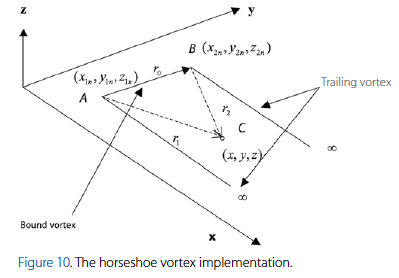
Equation 16 is the general expression for the calculation of the induced velocity for a finite length vortex segment. In addition, the horseshoe vortex is made up by the summation of the finite length vortex segment and two trailing vortices that extend to infinity. A general expression is required for the velocity induced at a point in space (x,y,z) by a horseshoe vortex. The derivation of this general expression is divided in three main parts that go in accordance with each vortex segment. Figure 10 illustrates the case for the horseshoe vortex with a general point in space with three spatial coordinates.

The vector definitions needed for the calculation of the velocity induced by the bound vortex segment at point C are given by the following expressions:

The velocity induced by the trailing vortices can be calculated using the semi infinite vortex case analysis. This vortex case calls for a new vector definition that recognizes a third point on the vortex filament that extends to infinity represented by point D. The new vector definitions will keep the same numbering notation used earlier for the explanation of the bound vortex. Figure 11 illustrates the new vector expression.

The derivation for the velocity induced at point C by the trailing vortex is the same as for the bound vortex. The only difference in this case is perceived when x3 goes to infinity. Taking this into consideration, the contribution of the trailing vortex is expressed as:

In general, the total velocity induced by a horseshoe vortex at a point in space C is given by the summation of the contribution of the bound vortex and the two trailing vortices. In fact, the general expression for this velocity is given by:

Equation 23 is the velocity induced at the mth control point by the horseshoe vortex representing the nth panel. The influence coefficient depends on the geometry of the nth horseshoe vortex and its distance from the control point of the mth panel (Bertin, J., & Smith, M., 1998). In order to find the total induced velocity at the mth control point induced by the 2N vortices, equation 23 is expressed as

Each control point lies within a horseshoe vortex representing a surface element. Hence, a lifting surface such as a wing is represented by a combination of these surface elements. The location of the horseshoe vortex and its control point is determined by a mathematical analysis described in the following section. According to (Bertin, J., & Smith, M., 1998), tradition has been to determine their locations by comparisons with known results. Their placement has become a rule of thumb in numerical panel methods.

Location of the Control Point and Bound Vortex
The location of both the control point and the bound vortex is determined not by a theoretical law, but instead by a placement that works well in accordance to theory. According to Bertin, J., & Smith, M. (1998), the control point of each panel is centered spanwise on the three-quarter chord line midway between the trailing vortex legs. Figure 12 illustrates the placement of the control point and the bound vortex.

The vortex filament of strength Γ positioned at the quarter chord location, induces a velocity at the control point cp given by

This result agrees with the infinite vortex filament case described earlier in sub-section “The Infinite Vortex Filament”. According to Bertin, J. & Smith, M. (1998), if the flow is to be parallel to the surface at the control point, the incidence of the surface relative to the free stream can be expressed as:

In order to solve for the unknown distance r, equation 25 calls for combined use of the Kutta-Joukowsky theorem and the results from thin airfoil theory. The combination of both relations gives the following result

Equation 25 is then substituted in equation 26; as a result, the unknown distance r can be solved as a function of the chord length.

Thus, the control point is located at the three quarter- chord location, and the bound vortex is located at the quarter-chord location. Both, the position of the bound vortex and the control point are functions of the chord length and the panel geometry.

Analysis and Application of the Boundary Conditions
The solution of the induced velocity at a control point in space by a horseshoe vortex is possible through the application of the boundary conditions. The vortex strength Γn in equation 24 represents the lifting flow field of the wing. In order to solve for this flow field, the surface is considered a streamline. The resultant flow is tangent to the wing at each and every control point. As a result, the component of the induced velocity normal to the wing at the control point balances the normal component of the free-stream velocity. The tangency condition yields the following relation.

where δm is the slope of the mean camber line at the control point and is the dihedral angle of the wing. Equation 28 can be simplified according to the shape of the airfoil section and the slope of the mean camber line. The tangency condition will give the solution for the system of simultaneous equations represented by equation 24. The unknown vortex strengths of each surface elements or panels are found through this solution.

Conclusion
Vortex lattice theory presents an alternative to different computational fluid dynamic methods. It is a quick technique that works well for the calculation of the lift coefficient and pressure distribution of a wing with angle of attack variation under conditions where there is no significant flow separation over a finite surface. It serves well as a method of computational fluid dynamics and can prove as an aerodynamic optimization technique that could extend its application to different Mach number regimes through the potential of adapting compressibility corrections to model flow. The use of Vortex Lattice Theory presents an opportunity for the aerospace engineer to come up with fast solutions for the calculation of aerodynamic coefficients where otherwise, the complexity of other computational fluid dynamic alternatives would have proven difficult and time consuming affecting the release and timeline of design elements crucial for the end project or result.

References

Abbot, Ira, Albert von Doenhoff. (1959). Theory of Wing Sections. New York: Dover Publications, Inc.

Anderson, J. (1998). Aircraft Performance and Design. New York: McGraw Hill.

Anderson, J. (2001).Fundamentals of Aerodynamics. New York: Mc- Graw Hill.

Bertin, J. & Smith, M. (1998). Aerodynamics for Engineers. New Jersey: Prentice Hall.

Chen, S. & Zhang, F. (2002). A Preliminary Study of Wing Aerodynamic, Structural and Aeroelastic Design and Optimization. AIAA-2002-5656.

Holst, T. (2005). Genetic Algorithms Applied to Multi-Objective Aerodynamic Shape Optimization. NASA/TM-212846.

Jackson, P. (2005). Jane’s All the World’s Aircraft. Cambridge University Press, UK.

Klatz, J. & Plotkin, A. (2001). Low Speed Aerodynamics. Cambridge University Press, Cambridge.

Mason, W.H. (1998). Aerodynamics of 3D Lifting Surfaces though Vortex Lattice Methods. Virginia Polytechnic Institute and State University. Retrieved from http://www.aoe.vt.edu/~- mason/Mason_f/CAtxtChap6.pdf>

McCormick, B.W. (1979). Aerodynamics, Aeronautics, and Flight Mechanics. New York: John Wiley & Sons.

Raymer, D. (1999). Aircraft Design: A Conceptual Approach. Reston: American Institute of Aeronautics and Astronautics, Inc.

Sivells, J. C. (1947). Experimental and Calculated Characteristics of Three Wings of NACA 64-210 and 65-210 Airfoil Sections with and without 2° Washout. NACA TN. 1422